Featured, Fundamentals, Spacecraft Attitude Dynamics

Spacecraft Attitude Kinematics

January 30, 2022

Attitude kinematics is the study of the rotational motion of an object without taking into consideration the forces or torques that started it. Attitude kinematics equations allow to predict and propagate the rotational motion of an object in time and are thus a very powerful tool. In this post they are examined and an example of their use is provided.

Introduction

Attitude kinematics studies how a reference frame changes attitude in time given its attitude parameters and angular velocity. In other words, the main goal is to understand the relationship between the derivative of the chosen attitude representation and the current attitude in a precise time step. No forces or torques are considered in this problem: in order to set in motion a point or to rotate a reference frame, energy must certainly be supplied in the form of forces or torques, but this concept is not examined in kinematics. Kinematics indeed studies the motion of an object without any considerations on the forces/torques that generated it, and for this reason it is also referred to as the geometric study of the motion.

[Fig. 1]: Example of an inertial and non-inertial reference frames in relative rotational motion

Attitude kinematics

The most important equation that is needed to derive attitude kinematics ones is the transport theorem, which is obtained by taking the derivative of a vector and writing it in two different reference frames. It states that:

$\bm{\dot{u}_a} = \bm{C_{ab}} ( \bm{\dot{u}_b} + [\bm{\omega_{ba}}]^\times \bm{u_b} )$

where $\bm{u}$ is a generic vector and $\bm{u_a}$ and $\bm{u_b}$ are its components in an inertial reference frame $\bm{A}$ and a non-inertial one $\bm{B}$ (represented with lower case letters in the equations). Finally, $[\bm{\omega_{ba}}]^\times$ is the cross product matrix form of the angular velocity of reference frame $\bm{B}$ with components expressed in frame $\bm{A}$ . The theorem links the derivative of a vector in a non-inertial reference frame and in an inertial one by means of a “bonus” velocity that must be added, the term $[\bm{\omega_{ba}}]^\times \bm{u_b}$ , which arises when the relative angular velocity is different from zero.

The transport theorem can be leveraged to obtain the expression for the derivative of the rotation matrix between two frames, which represents the attitude kinematics equations. The resulting expression is:

$\bm{\dot{C}_{ab}} = \bm{C_{ab}} [\bm{\omega_{ba}}]^\times$

which relates the derivative of a rotation matrix with the current rotation matrix and the angular velocity. When using quaternions, the expression changes to:

$\bm{\dot{q}} = \left[\begin{array}{c} \frac{1}{2}(\eta\bm{I}_{3,3} + \bm{\epsilon}^\times) \\ -\frac{1}{2} \bm{\epsilon}^T \end{array}\right] \bm{\omega_{ba}}$

which again relates the derivative of the quaternion vector with the quaternion vector itself and the angular velocity.

Another important equation can be retrieved using the transport theorem, written in vector form for linear velocity $\bm{\dot{u}}$ and acceleration $\bm{\dot{v}}$ :

$\bm{\dot{u}} = ( \bm{\mathring{u}} + \bm{\omega_{ba}}\times\bm{u} )$

$\bm{\dot{v}} = ( \bm{\mathring{v}} + \bm{\omega_{ba}}\times\bm{v} )$

where $\bm{\mathring{u}}$ denotes the hollow derivative, which is the derivative of a vector taken in a non-inertial reference frame (such as frame $\bm{B}$ ). By combining those equations the Coriolis kinematic equation is obtained as:

$\bm{\dot{v}} = \bm{\mathring{v}} + 2 \bm{\omega_{ba}}\times \bm{\mathring{u}} + \bm{\omega_{ba}}\times \bm{\omega_{ba}}\times\bm{u} + \bm{\mathring{\omega}_{ba}}\times \bm{u}$

or, using components:

$\bm{\ddot{u}_a} = \bm{C_{ab}} ( \bm{\ddot{u}_b} + 2 [\bm{\omega_{ba}}]^\times \bm{\dot{u}_b} + [\bm{\omega_{ba}}]^\times [\bm{\omega_{ba}}]^\times \bm{u_b} + [\bm{\dot{\omega}_{ba}}]^\times \bm{u_b})$

This last expression, similarly to the transport theorem, relates the acceleration of a point seen from an inertial and a non-inertial reference frame.

Methods

In the following sections an example of integration of the attitude and Coriolis kinematics equations is provided. In order to carry the integration, the equations have been reduced to a system of first order differential equations first. The variables vector is composed as follows:

$\bm{y} = \left[\begin{array}{l} \bm{y_1} \\ \bm{y_2} \\ \bm{y_3} \\ \bm{y_4} \\ \bm{y_5} \end{array}\right] = \left[\begin{array}{l} \bm{q_{BI}} \\ \bm{r_{P,B}} \\ \bm{v_{P,B}} \\ \bm{r_{P,I}} \\ \bm{v_{P,I}} \end{array}\right]$

where $\bm{q_{BI}}$ is the quaternion vector representing the body reference frame $\bm{B}$ attitude in the inertial $\bm{I}$ reference frame. $\bm{r_P}$ and $\bm{v_P}$ are the position and velocity vectors of point $P$ and their components can be written in the inertial $\bm{I}$ frame or non-inertial body fixed frame $\bm{B}$ as needed. The system of first order differential equations is then:

$\bm{\dot{y}} = \left[\begin{array}{l} \bm{ \dot{y} _1} \\ \bm{ \dot{y} _2} \\ \bm{ \dot{y} _3} \\ \bm{ \dot{y} _4} \\ \bm{ \dot{y} _5} \end{array}\right] = \left\{ \begin{array}{lr} \bm{ \dot{y} _1} = f(\bm{q_{BI},\omega_{BI}})\\ \bm{ \dot{y} _2} = \bm{y_3}\\ \bm{ \dot{y} _3} = \bm{a_{P,B}} \\ \bm{ \dot{y} _4} = \bm{y_5} \\ \bm{ \dot{y} _5} = \bm{C_{IB}}(\bm{q_{BI}}) ( \bm{a_{P,B}}+ 2 [\bm{\omega_{BI}}]^\times \bm{y_3} + [\bm{\omega_{BI}}]^\times [\bm{\omega_{BI}}]^\times \bm{y_2} +[\bm{\dot{\omega}_{BI}}]^\times \bm{y_2}) \end{array} \right.$

where the function $f(\bm{q_{BI},\omega_{BI}})$ represents the quaternion kinematic equations, $\bm{ \omega_{BI}}$ is the angular velocity of frame $\bm{B}$ with respect to $\bm{I}$ and $\bm{a_{P,B}}$ is the non-inertial acceleration of point $P$ .

The equations have been numerically integrated with both Matlab ode45 and ode113 with identical results. In order to ensure the integrity of the computations, the following tests have been performed:

The norm of the quaternion vector $\bm{q_{BI}}$ is always equal to one. A normalization procedure is performed during each integration step to ensure that this requirement is met.
The absolute values of the distance vectors $\bm{r_{P,I}}$ and $\bm{r_{P,B}}$ must be equal, since the origin of the two reference frames $\bm{I}$ and $\bm{B}$ are the same. The modulus of $\bm{r_{P,I}}$ is compared to the modulus of $\bm{r_{P,B}}$ and $\bm{C_{IB}}\bm{r_{P,B}}$ .
Finally, the inertial velocity $\bm{v_{P,I}}$ must be equal to its analytical conterpart, which is obtained using the transport theorem as $\bm{C_{IB}}([\bm{\omega_{BI}}]^\times \bm{r_{P,B}}+\bm{v_{P,B}})$ .

Results and discussion

After defining the system of equations for attitude kinematics equations, some parameters and initial conditions are needed to start the simulation. The non-inertial acceleration of point $P$ and the relative angular velocity between frames $\bm{I}$ and $\bm{B}$ have been arbitrarily imposed as follows:

$\bm{a_{P,B}}(t) =\left[\begin{array}{c}0.02\\0\\0\end{array}\right] (\frac{m}{s^2})$

$\bm{\omega_{BI}}(t) = \left[\begin{array}{c}0.06 t\\0\\0\end{array}\right] (\frac{rad}{s})$

While the initial parameters have been initialized as:

$\bm{r_{P,B@t0}} =\left[\begin{array}{c}0\\0\\1.5\end{array}\right] (m)$

$\bm{v_{P,B@t0}} = \left[\begin{array}{c}0.25\\0\\0.0625\end{array}\right] (\frac{m}{s})$

$\bm{q_{BI@t0}} =\left[\begin{array}{c}0\\0\\0\\1\end{array}\right] (-)$

With these conditions the particle undergoes linear motion along the $z$ axis of frame $\bm{B}$ and uniformly accelerated motion along the $x$ axis, as shown in [Fig. 2]. The motion that is observed from frame $\bm{I}$ takes the shape of an expanding helix trajectory. [Fig. 3] and [Fig. 4] reproduce the first 21 seconds of motion when observed from frame $\bm{B}$ and $\bm{I}$ respectively.

[Fig. 2]: Position of point $P$ in $\bm{B}$ and $\bm{I}$ frame

[Fig. 3]: Trajectory of point $P$ in frame $\bm{B}$ . Acceleration components vectors not to scale

[Fig. 4]: Trajectory of point $P$ in frame $\bm{I}$ . Acceleration components vectors not to scale

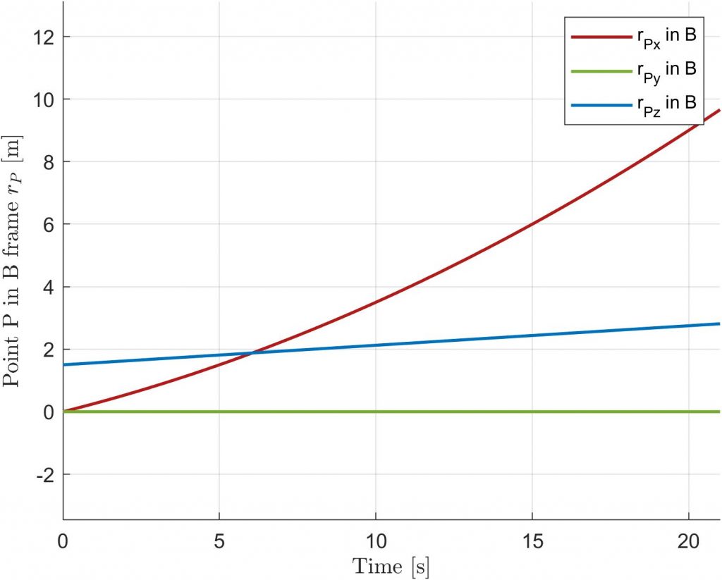
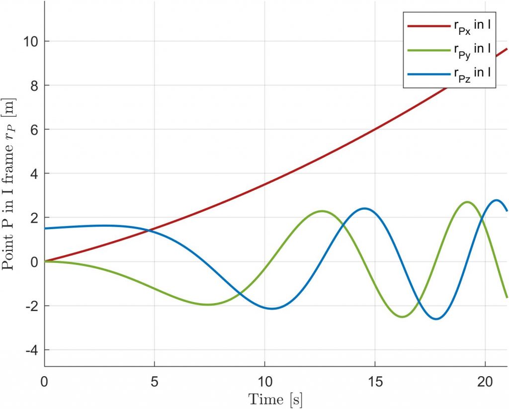
[Fig. 3] and [Fig. 4] also depict the various accelerations that point $P$ experiences depending on the selected reference frame. There are four major contributions to the inertial acceleration $\bm{a_{P,I}}$ of point $P$ :

Non inertial acceleration $\bm{a_{P,B}}$ : this is the acceleration of point $P$ in reference frame $\bm{B}$ . As such, it is responsible for causing the accelerated motion of point $P$ that occurs in frame $\bm{B}$ .

Coriolis acceleration $2 [\bm{\omega_{BI}}]^\times \bm{v_{P,B}}$ : Coriolis acceleration is present only if point $P$ has a non null velocity $\bm{v_{P,B}}$ in frame $\bm{B}$ . If that occurs, the acceleration direction is perpendicular to both the angular velocity vector and the velocity vector.

Centripetal acceleration $[\bm{\omega_{BI}}]^\times [\bm{\omega_{BI}}]^\times \bm{r_{P,B}}$ : this acceleration is always present in a rotating reference frame and its value is proportional to the distance vector. By definition, the centripetal acceleration is perpendicular to the angular velocity vector and is also contained in the plane defined by the angular velocity vector and the distance vector.

Transversal acceleration $[\bm{\dot{\omega}_{BI}}]^\times \bm{r_{P,B}}$ : the transversal acceleration is caused by a variation in time of the angular velocity. When an angular acceleration is indeed present, the transversal acceleration is generated too, perpendicular to both the angular acceleration vector and the distance vector.

In [Fig. 5] the absolute values of the example taken into consideration in this section are shown.

[Fig. 5]: Acceleration components vectors of point $P$ in frame $\bm{I}$

Conclusion

In this post attitude kinematics equations and Coriolis kinematics equations have been explored and an example of their integration has been provided. The attitude kinematics equations have been used to relate the relative attitude of an inertial and a non-inertial reference frames. A generic point $P$ has been set in an accelerated motion in the non-inertial reference frame and, by using Coriolis kinematics equations, its inertial trajectory has been recovered. The four components of the inertial acceleration have been computed as well, and their contribution and meaning in the overall total acceleration have been explored.